When Basic Reliability Models Fall Short

Often times reliability models are straightforward and routine, and a standard model is sufficient to show compliance with reliability requirements. However, there are times when a standard model will not provide the needed answers; so how do we successfully address reliability of systems with complex architecture and associated definition of system failure? Over the years, ALE has encountered many unique challenges where routine reliability models and approaches are inadequate and do not provide truly meaningful insights. The following provides a generalized discussion of a more recent real world example where ALE reliability engineers developed an in-house, tailored analysis tool to assist a customer in demonstrating reliability compliance given their “unique” system design and performance requirements.

The methodology used in this reliability analysis is based on Monte Carlo simulation theory. Monte Carlo simulation is a standard methodology used in many mathematical, engineering, and financial areas such as optimization, numerical integration, and selecting from probability distributions. Many good resources are available via a quick internet search to provide more information about Monte Carlo simulation.

sample problem

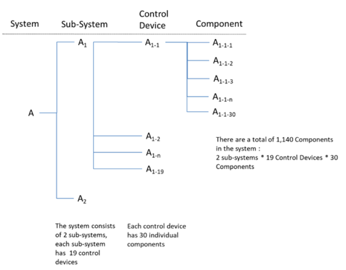
In this particular example, the results of a standard Monte Carlo simulation would not accurately model actual application of the system under development. The customer’s system is designed to allow non-linear degradation in performance over time while the overall system continues to operate, successfully satisfying key performance parameters. The system (A), illustrated in Figure 1, consists of 2 sub-systems (A₁ and A₂), each independent of the other and each contain a set of controllers (A_1-1 – A_1-19, A_2-1 – A_2-19). Each of the 38 independent controllers control a set of 30 components (A_1-1-1 – A_1-1-30, A_1-2-1 – A_1-2-30, etc.), resulting in a total of 1,140 individual components in the system. Failure of a higher-level subsystem results in a loss of functionality of the lower level elements which they control, but the remainder of the system remains functional.

An approach was needed that would simulate the occurrence of failures of low-level hardware (i.e. sub-systems, controllers, and/or components) over time and calculate the resulting level of system performance degradation. As shown by the system diagram, a failure of one sub-system will result in 570 components being non-operational (19 controllers * 30 components = 570 components). Similarly, a failure in one controller will result in 30 components being non-operational. As long as the number of functional components remain above the minimum required, the system will satisfy the performance requirements and the simulation will continue. When the model indicates the system has accumulated more than the pre-established maximum number of failures in any combination of sub-system(s), controller(s), and components, the simulation categorizes the system as failed.

Hourly probabilities associated with hardware failures were calculated using failure rates developed as part of the system hardware reliability prediction effort using standard reliability methods. To determine if a failure has occurred, the simulation generates a random number between zero and one, which is used as the seed probability. The model compares the seed to the system failure probability and makes a determination as to whether the entire system is failed. If the system is determined not to have failed, a new seed is generated and compared to the failure probability of the first sub-system. This iterative process continues through the second sub-system, all device controllers, and all components, with the program maintaining a running record of the failed components. The resulting component failures are summed to determine whether the system is still considered functional. If the system is functional, the time period is incremented, and the process repeated until the system fails. Upon system failure, relevant data, including time of failure and the number of failed components, is logged and the system reset to a fully operational state for the next iteration.

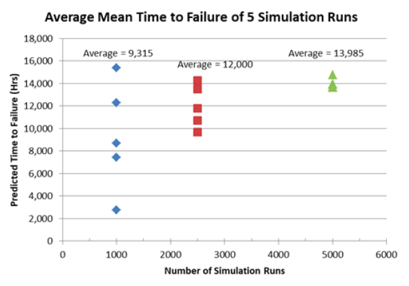
As the number of simulation runs are increased, the average failure time converges asymptotically with less variance between runs as illustrated in Figure 2. This average failure time was used to calculate the predicted failure rate of the system using standard reliability equations. Figure 2 shows that running the simulation 5 times at 5,000 iterations each provided a mean time to failure of 13,985 hours. The confidence in this result is much higher than running the model for 1,000 or 2,500 iterations. However, there is a tradeoff in increasing the number of iterations with the significant increase in computing time. Graphing the results will help identify the optimal number of iterations at which increasing the number of iterations has a minimal change to the average failure time.

CONCLUSIONS

In developing the simulation as a stand-alone application, ALE leveraged our experience and knowledge of reliability analysis methodologies to address the real world challenge of demonstrating compliance with performance requirements for our customer; a feat not achievable using standard reliability models. Had the model demonstrated the system was unlikely to meet performance requirements, additional insights into system architecture could be obtained to support trade studies of potential design changes towards increasing system reliability and satisfying program requirements. Data recording aspects of the model were further customized to record individual component failures over time. This data was used to provide a real-time visual model that illustrated the state of the system throughout the simulation, a level of customization that would not be achievable using a prebuilt simulation model.

Article Authored by Rodney Benson